1.1 – Another project on private returns of education?

1The main idea behind the literature on education and the labour market is that better educated workers receive an education premium, resulting to higher earnings. We go beyond this well established evidence and raise the question of other potential benefits of education. First we ask whether better educated workers enjoy less unemployment or higher labour market participation. The next question was how persistent are education benefits and could they imply significant longer duration of careers for the high skilled? And finally, could parental labour market outcomes influence youth educational attainment making it a two-way relationship? These three questions resulted into three different thesis’ sections, a summary of which is presented here.

2The three sections deal with “schooling”, the human capital an individual acquires usually from the age of five or six until adolescence or early adulthood. We have put the individual at the centre of our research, and we follow throughout his education and working years. It is a micro-level research project, and does not cover issues such as the contribution of education to growth or the social benefits of education. All three sections discuss individual decisions. The educational system, the level of wages, and unemployment benefits, the unemployment rate are exogenously set. Individual ability is also exogenous.

1.2 – Extending the Becker/ Mincer approach

3This project has its roots in the intellectual tradition initiated by Mincer (1958) and Becker (1964), but extends it to account for issues that have gradually become more relevant such as the effect of education on lifelong labour supply/retirement decision.

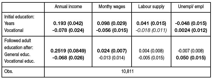
4This literature on the wage premium (Ashenfelter (1978), Card (1999), Ashenfelter et al., 1999) was developed at a time when the economic benefits of education could be restricted to wages. As the labour market conditions worsened, the question became whether education can also protect against unemployment and inactivity. As soon as from the late 1970’s Ashenfelter & Ham (1979) noticed that the benefit of education can be decomposed to an income and a time effect. Much later, Mincer (1991a, b) decomposes unemployment rates into unemployment incidence and unemployment duration. Better educated workers have better probabilities to find a suitable job and remain attached to it, while they face less risk to become unemployed.

5The assumption of homogeneous and undifferentiated human capital proved another restrictive assumption, especially for continental Europe with stratified education systems. While US evidence show that vocational high-school courses improve future labour market outcomes for those who choose not to follow tertiary education (Bishop & Mane, 2004; Mane, 1999), research in Europe compares vocational and academic education and the later proves to be more efficient and rewarding in labour market terms (Conlon, 2001; Dearden et al., 2000).

6There has been a great concern lately on the effects of ageing in Europe and its labour market implications (Boersch-Supan (2001), Blanchet, (2001)). However, little have been said on how education can affect the moment of individual retirement, probably because many believe that education effects diminish and gradually disappear after entering the labour. We felt however that there might be significant differences in the retirement behaviour between high and low educated individuals, due to heterogeneity in earnings from work, and retirement incomes. Social security schemes might increase or alleviate these differences.

1.3 – Why is Belgium an interesting case?

7To extend the Becker/Mincer analysis of education we worked with Belgian data. Belgian educational system delivers heterogeneous forms of human capital (i.e. different tracks). It has large participation rates in vocational and technical programmes (both in secondary and tertiary education), higher from the EU19 and the OECD average (Table 1).

Table 1

Upper secondary enrolment patterns, by programme destination and programme orientation, 2006 (%) [2]

By programme destination By programme orientation ISCED 3A2 ISCED 3C General Vocational Combined school and work-based Belgium 49.4 50.6 30.6 69.4 3.5 EU19 70.1 24.1 46.7 47.8 16.3 OECD 69.8 26.0 53.8 44.0 15.2

Upper secondary enrolment patterns, by programme destination and programme orientation, 2006 (%) [2]

8School performance is higher in general than in vocational education (Table 2). The over 100-point difference in maths and science performance between the two tracks is very large compared to the OECD average and one of the highest among European countries and persists even after controlling for pupils’ socioeconomic background (ESCS).

Table 2

Performance of 15 year-olds on the PISA science and mathematics scales

General programmes (A) Vocational programmes (B) (A)-(B) (A)-(B) after controlling for ESCS Maths (2003) Belgium 585 469 116 78 OECD 510 466 45 27 Science (2006) Belgium 558 458 100 78 OECD 509 473 35 24

Performance of 15 year-olds on the PISA science and mathematics scales

9Better educated workers perform better in the labour market, in terms of earnings but also in terms of (un)employment rates. According to OECD (2008a), wage premia in Belgium have been relatively stable during the past decade, but, the employment premium has risen. This tentatively suggests that Belgium is ideal to explore the non-wage benefits associated to education.

10A final reason behind our country choice is simply the novelty of our analysis in the Belgian context. Up to date most works focus on programme and policies evaluation (Cockx & Ries, (2004)), special features of the Belgian labour market (D’Addio & Nicaise (2003)), or policy reforms and their effectiveness (Desmet et al. (2003)).

11The dataset we use is the Panel Study of Belgian Households (PSBH) (1992-2002). The survey was launched in 1992 jointly by the Universities of Liege (for Wallonie) and Antwerp (for Flanders). From 1994 till 2002 it became part of ECHP, the European Household Panel. It includes three separate questionnaires, for adults, households and children 0-16 years old. It provides rich information on income, employment and education household composition. Its eleven waves also allow us to follow persons and households and examine transitions and changes in their lives.

2.1 – Introduction

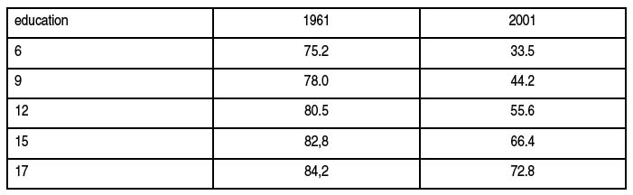
12Belgium is a country with an extensive social security system which comprises transfers earmarked for families with children, such as child allowances or higher unemployment benefits for those with dependent children. Significant resources are also spent on combating parental unemployment.

13Regarding the success of these programs, Belgium seems to have been successful at combating child poverty (child poverty was at 10 percent of the total population in 2005 compared to 11.0 percent for EU-26 and 12.4 percent for OECD (OECD, 2008b)).

14Here we discuss a possible causal relationship between parental income and employment with educational attainment, which in its turn is a crucial determinant of the long-term employment and income prospects for children when they will enter labor market. For Belgium, a significant factor for childrens’ educational attainment is the sorting between the qualification (vocational and technical education) and the transition (general and artistic education) track that usually occurs around the age of 14. In principle it is considered to be a neutral choice, however in reality it is a strong predictor of continuing and successfully completing tertiary education (Eurostudent, 2005). Given the early age of youth, sorting can be influenced by parental background, including income (Checchi & Flabbi, 2007; Dustmann, 2004). Even in a tuition-free system such as the Belgian one, poorer students could choose the qualification track for example, to enter the labor market sooner. Poorer or unemployed parents could also persuade children to opt for shorter qualification tracks in order to be prepared to enter labor market at the end of compulsory education, or they themselves could lack the motivation to persuade their children to follow more ambitious education tracks (Barron, 2009; Gregg et al., 2008).

15However, there exist several reasons why the relationship between parental income, employment and school choices is not causal. Parents with high income also have higher education, reflecting differences in ability or motivation that might be passed on to their children (Chevalier et al., 2005). Social relations and pressure from peer groups can also inuence schooling decisions (Mohanty & Raut, 2009).

16We try to capture causal effects by comparing school choices made by siblings in different points in time, thus we cancel out motivation or ability factors (Levy & Duncan, 2000). We dismiss the idea of a causal relationship once we control for unobserved family characteristics which is in line with similar works that discuss university attendance (Vandenberghe, 2007; Dearden et al., 2004) or track choice in Germany (Tamm, 2008). By contrast, the labour market status of parents could matter.

2.2 – Choosing between different educational tracks in Belgium

17Education in Belgium is primarily the responsibility of the Communities. The structure of the education system is very similar between the Communities and also resembles those of Central Europe. One of its main features is the existence of multiple tracks and sorting of students at a very early age.

18After completing primary education, and providing they have not repeated any grades that far, young pupils enter secondary education around the age of 12. After two common years of studies they are asked to choose among two tracks. The transition track (general and artistic education) provides general and academic knowledge preparing for tertiary education. Since pupils in the transition track usually continue with tertiary education, they also get on average more years of schooling. This in general implies higher earnings (Belzil (2004); Heckman et al. (2003)), lower unemployment and less time spent in inactivity (Mincer, 1991a). The qualification track (technical and vocational) provides professional qualification in several fields (Eurydice, 2001). Many pupils enter this cycle after 14 as a result of poor performance. Although in theory it does not exclude students from tertiary education this is rarely the case.

19School systems with very early tracking have been held partly responsible for low mean and high variance in literacy scores of 15-year-olds in the PISA 2000 assessment (OECD, 2000). Furthermore, some works argue that early sorting of students also leads to low educational mobility and could be held responsible for a strong association between educational attainment and labour market inequality (Checchi & Flabbi, 2007).

2.3 – The sample and estimation method

20We seek to estimate the effect of family income and parental activity on young pupils’ educational choices once we have controlled for family background variables F and child characteristics C. We estimated linear probability models for their simplicity and because they give good estimates of the partial effects near the center of the distribution compared to nonlinear estimates (Wooldridge (2001)). To correct for bias resulting from unobserved family factors we used family fixed effects models ( [3]) (within-families differences).

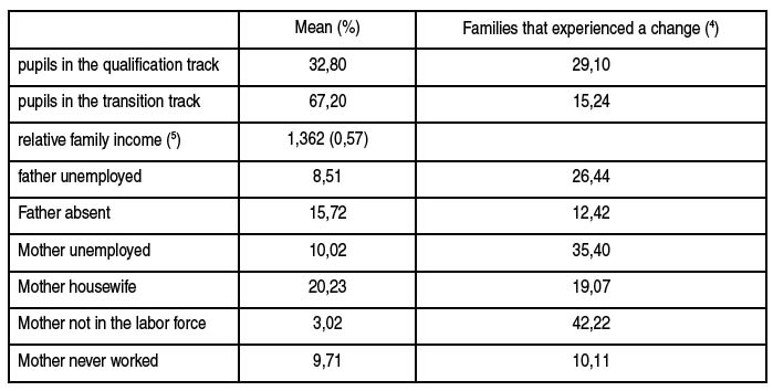
21The sample included 402 families with at least 2 children in secondary education during the 11 waves of the PSBH (897 observations). For each of the children we observed their track choice and family income and employment at that specific moment (Table 3). We used as controls children’s characteristics (sex, age, siblings’ birth order, and the number of grade repetitions as a proxy for school performance), and family background (parental education and nationality, region of residence and family wealth). We catch possible time effects with wave dummies.

Table 3

Track choice, family income and employment [4] [5]

Mean (%) Families that experienced a change (4) pupils in the qualification track 32,80 29,10 pupils in the transition track 67,20 15,24 relative family income (5) 1,362 (0,57) father unemployed 8,51 26,44 Father absent 15,72 12,42 Mother unemployed 10,02 35,40 Mother housewife 20,23 19,07 Mother not in the labor force 3,02 42,22 Mother never worked 9,71 10,11

Track choice, family income and employment [4] [5]

(percentages)

2.4 – Results and policy implications

22In cross-section models, family income has a strong negative effect on track choice, even after controlling for children’s and family characteristics. One unit positive change in the relative position of the household in the income distribution decreases by 35 percent the probability of following the qualification track, after controlling for observable characteristics (Table 4). These results are different from Carneiro & Heckman (2002) and Dearden et al. (2004), where income effects become negligible and statistically insignifiant after controlling for observable characteristics. On the other hand, Tamm (2008) is in line with our findings.

Table 4

Family income and track choices [6] [7] [8]

Model 1 (6) Model 2 (7) Model 3 (8) Income -0.504 (0.063) -0.476 (0.061) -0.352 (0.067) Income square 0.080 (0.014) 0.076 (0.014) 0.070 (0.013) Obs 897 897 897

Family income and track choices [6] [7] [8]

(cross-section)
(in bold): statistically significant at 95 percent confidence level

23School performance, measured by no grade repetitions has a strong negative effect on choosing the qualification track. Low-educated parents increase the probability of children following the qualification track, with mothers’ education having a larger effect on track choices, implying a greater impact on children’s school performance and preferences.

24When we control for unobserved family characteristics (sibling fixed effects), the income effect remains negative, however it shrinks considerably and is no longer statistically significant. This implies that children face no short run constraints due to low income. Our results are in line with Tamm (2008). We can then interpret findings in both works as a proof of no causal relationship between income and track choice.

25We get different results once we regress track choice on parental activity (Table 5). When the father is unemployed, there is a greater probability that children will follow the qualification track. This effect remains significant (at 90 percent confidence level) even after controlling for income. On the other hand we get a positive effect on track choice when the mother stays at home, implying that quality time spent with children has a positive influence (non-significant coefficients are probably due to small sample). Our results are somewhat different from those in Nörberg-Schönfeldt (2008). They find that full-time working mothers as well as nonworking mothers have negative impact on their children’s school performance, compared to part-time working mothers; these differences between them and us, could just reflect different model specifications. However, the general idea is that a mother affects her children’s choices and school performance through income and the time she spends with them. The one effect offsets the other (the more she works, the more she can provide but also the less she interacts with her children) and the final result is ambiguous.

Table 5

Parental activity and track choices [9] [10] [11]

Model 4 (9) Model 5 (10) Model 6 (11) Unemployed father 0,188 (0,110) 0,208 (0,127) 0,181 (0,108) Unemployed mother -0,089 (0,081) -0,118 (0,083) -0,046 (0,081) Housewife mother -0,143 (0,122) -0,142 (0,123) -0,189 (0,116) Mother never worked -0,371 (0,195) -0,391 (0,197) -0,366 (0,187) Observations 897 897 897

Parental activity and track choices [9] [10] [11]

(FE models, st.errors in parenthesis)
(In bold): Statistically significant at 95 percent confidence level
(in italics): Statistically significant at 90 percent confidence level

26In general the results suggest that mother’s activity affects children’s education mainly in the long run compared to the effects of father’s activity which are mainly in the short run (track choice is affected by father’s activity at that point in time), while income effects are negligible. Therefore income interventions at the age of track choice might have minimal or no results at all. Alternatively, increasing father’s employment can improve track choices in the short run.

3.1 – The multiple dimensions of education

30We wanted to create variables to measure the duration of schooling, but also to capture qualitative aspects of education such as the curriculum, specific features of the educational system and educational reforms.

31To this end we examined thoroughly the Belgian education system, its specificities due to the federal nature of the state, the cycles of education (primary, secondary, tertiary), two major educational reforms, one in 1971 that changed the structure of secondary education and one in 1990 that affected tertiary education. Finally we distinguished between general and vocational school tracks and also included in the analysis post-school vocational courses (offered at workplace or elsewhere e.g. ORBEM).

32Depending on the questions asked the relevant literature delivers different results. Evidence from the US (Mane (1999)) suggests that pupils who do not continue to college, do considerably better when they follow a vocational high-school curriculum. On the other hand, European (including UK) surveys report extra gains for individuals with academic qualifications (McIntosh, 2004; Conlon, 2001). However, there is the argument that better performance in the labour market is not a result of academic qualifications, but rather an indication of self-selection bias, since abler individuals usually follow general education (Malamud & Pop-Eleches, 2008).

33Evidence also suggest that education benefits depend on several factors other than duration and type of schooling, such as successfully completing a course, the field of studies and its relevance to the labour market and the sector (Grubb, 1997; McIntosh, 2004).

3.2 – Monthly or annual earnings?

34Crucial to the analysis is the choice of a measure of earnings, which is however often dictated by necessity (available information on datasets) (Card, 1999).

35Reported effects of schooling on annual earnings are usually higher than the effects on monthly or hourly earnings (Card, 1999; Mincer, 1974), since annual income is the product of hourly wages, hours worked per day, and days worked per year. Going a step further, an individual receives income a) when he is in the labour market i.e. is not in education or retirement and b) when he is not unemployed.

36Employment surely depends on education, otherwise, the effects of education would be the same, no matter the time dimension of income.

37Usually the education/working time relationship is positive either because labour supply increases with schooling or because more educated individuals become less frequently unemployed and/or spend less time in unemployment. Both of these explanations are plausible (Table 6).

Table 6

Labour force participation (LFS) and unemployment rates by education and gender, Belgium, 25-64 year olds (2001)

Education Below up-per secondary (?12yrs) Upper sec-ondary and post-secondary (12-14 yrs) Tertiary non-university (13-14 yrs) Univer-sity and post-graduate(? 18yrs) All levels LFS rates Males 69 87 91 92 81 Females 39 69 81 84 60 Unemployment rates Males 7.4 4.4 2.5 2.5 4.8 Females 10.4 6.9 2,4 3.8 6.3

Labour force participation (LFS) and unemployment rates by education and gender, Belgium, 25-64 year olds (2001)

38Education improves labour market experiences via technological changes (Nickell & Bell, 1995), screening from employers (Holzer, 1996), more effcient on- and off-the-job searching (Mincer, 1991a), psychological and sociological reasons (discouragement and exit from labour force for less skilled workers, family decisions such as the raising of children). It is interesting to estimate the gap between education effects on annual and monthly earnings and see which part is due to higher labour force participation and which part to less unemployment.

39Among the first to discuss these issues were Ashenfelter & Ham (1979) (A&H), whose model we use here. They assume that labour supply (h*) is the sum of employed (h) and unemployed (u) months, i.e. h*= u+h. All months spent in activities other than in a job or in unemployment are assumed as a part of an individual’s decision not to offer his labour supply. This holds as long as no restrictions such as compulsory schooling or compulsory military service exist.

40With a monthly wage w, desired earnings are then:

41

42where wh are annual realised earnings from work and u/h is the fraction of unemployment to employment months. By taking logs and differentiating with respect to schooling S the relationship becomes:

43

44Equation (2) decomposes the effect of schooling into its parts, i.e. the effect of schooling on wages, labour supply and u/h. Assuming that wh, w, h* and u/h are linear functions of schooling and a vector x of explanatory variables (equation (3)), any consistent estimates of ?’s would estimate the gap between education returns on annual and monthly earnings and determine its source.

45

46Any consistent estimates of the return to schooling in (3) will satisfy the relationship

47

48which is equivalent to (2). Equation (4) gives four possible cases that explain the gap between monthly and annual earnings. The first is the trivial one

3.3 – The sample and estimation techniques

49We use longitudinal data, which, compared to cross section, allow for control for omitted or unobservable individual specific effects. However, we cannot use any of the two traditional panel data estimators (fixed- and random-effects). With FE our main variable schooling is eliminated from the transformation of variables as deviation from the mean, as it is time invariant. RE produces inconsistent estimates if schooling is correlated to unobserved ability (a plausible assumption in this kind of models). Hausman & Taylor (1981) (HT) have then proposed an instrumental variable estimator that produces consistent estimates for time invariant variables. The idea behind HT is that control variables are divided into four groups depending on their time variability and their correlation to unobserved effects. Appropriate estimation techniques are used to produce estimates for each group. The drawback is that we need to make assumptions as to which control variables are exogenous; this can prove to be a tenuous task and here we omit all econometric details.

50We use data from years 1995-2001 of the PSBH. The sample includes males and females 18-65 years old, who have completed school and are at least one year working or unemployed. This left us with 10,811 observations (2,765 individuals).

51We use four variable groups:

1. The education group: years of (school) education, general and vocational, and after-school vocational education.
2. The income group: net annual income and monthly wages.
3. The time variables group: months in employment, unemployment and labour supply.
4. The control variables group: Marital status, age cohort, health, experience and experience square, sector of employment, profession and region (time-variant) and sex, nationality, father and mother education (time-invariant).

52An individual with primary education spends around 4.5 less days per year in the labour market compared to a university graduate. He also faces about 9% higher unemployment to employment (u/h) ratio. Again individuals with vocational education have higher u/h ratios, but we see no significant differences in labour supply.

5341.16% of the sample has followed after school vocational education. Workers with higher-than-average schooling engage more often in after school vocational education and training; a first indication that initial and after-school education are complements. Most workers follows courses organised at school or other academic establishment (18.66%).

54Most of individuals in the sample are married, have good health, are Belgian citizens, age 30 to 45, they work in the services sector and live in the Flemish region.

3.4 – Estimation results

55Estimation results (Table 7) show strong and significant effects of education on income and employment time.

Table 7

Estimation results using HT estimators

Annual income Monthy wages Labour supply Unempl/ empl Initial education: Years 0.193 (0.042) 0.098 (0.029) 0.041 (0.015) -0.048 (0.015) Vocational -0.078 (0.024) -0.056 (0.015) -0.018 (0.011) 0.0024 (0.012) Followed adult education after: General educ. Vocational educ. 0.2519 (0.0849) -0.068 (0.026) 0.024 (0.007) -0.013 (0.014) 0.004 (0.008) -0.005 (0.015) -0.007 (0.008) 0.050 (0.015) Obs. 10,811

Estimation results using HT estimators

(st. errors in parentheses)
(in bold): statistically significant at 95 percent confidence level
(in italics): statistically significant at 90 percent confidence level

56For all estimated coefficients, equation (4) approximately holds. For example, applying (4) to education coefficients, leaves us with (0.193 – 0.098 – 0.0409 + (-0.048)) = -0.0061, a very small and not statistically different from 0 difference. Hence the initial hypothesis that the effect of education on earnings is decomposed to the effect on monthly wages and employment time is confirmed.

57General education produces better incomes, less unemployment, and more time in the labour market. These results are in line with European surveys that speak in favour of general education (Dearden et al., 2004; Cooke, 2003; Conlon, 2001).

58The effects of vocational after school education vary considerably depending on completed schooling ( [12]). There are considerable gains from after school education for those secondary education or university graduates, implying that general and adult education are complements. Similar results are found in Cooke (2003).

59The effects of initial general education are higher for women than for men for all of our four models. Education is more important for participation in the labour market for women than it is for men but it does not change wages of men and women. Vocational initial education implies lower wages and consequently earnings for both genders, but it hurts women more.

60We also estimated separate models for three age cohorts: those born before 1945, between 1946 and 1965 and between 1966 and 1983. The main conclusion was that education affects mainly younger cohorts, both in terms of earnings and time.

61Finally we performed separate regressions for the three Belgian regions (Wallonie, Flanders and Brussels). Initial general education has strong positive effects for those who live in Brussels and in Flanders, while effects for Wallonia are much smaller. Moreover, in Wallonia there is a much stronger negative effect of initial vocational education compared to Flanders. The return of after school vocational education is higher for Wallonia, slightly lower in Flanders and much lower in Brussels.

3.5 – Conclusions

62Not many studies estimate the effect of education on earnings and employment time in the way that it is done here. We have shown that education improves significantly not only the income of individuals but also the experiences they have in the labour market. This improvement is much larger than traditional estimation methods predict.

63Comparing general and vocational education, the evidence speak in favour of general schooling, both in terms of income and employment, even after controlling for individual ability. Vocational education and training seems a better choice after school. The assumption of complementarities between initial and after school education is also confirmed.

64Individuals should be encouraged to receive education to enjoy higher income and better labour market experiences. However the choice between different types of education also matters.

4.1 – Introduction

65Modern societies are getting older as a result of dramatic drop in birth rates and improved medical and living conditions that raised the average age expectancy. According to the European Commission, from 2010 the EU15 will start experiencing a fall in the total working age population and from 2020 a fall in the total population (EC, 2003a). At the same time, employment and labour force participation of older workers drops because of generous retirement benefits and other retirement incentives. Among European countries, Belgium holds one of the last positions (EC, 2003a) in employment and participation of older workers.

66These demographic changes cause major burdens on social security and medical care systems (EC, 2003a), significant wage/ productivity gaps (Hellerstein et al., 1996), increased labour costs, drops in the productivity, and uncovered vacancies (EC, 2003b). For policy makers the answer to these problems is to increase labour force participation and employability of older workers (EC, 2003a, b, 2002). They propose education and training as means to keep older workers longer in the labour market.

67In Echevarria & Iza (2006), individuals engage in education because they discount future wages and future pension benefits. Then, the better educated enter the labour market later and they prolong their stay in education, because of higher discounted wages and pensions. In our case all workers enter the labour market at the same time, but higher ability workers have accumulated higher human capital. This is crucial, as in our model, postponing retirement implies a true increased duration of working lives rather than a later age of leaving the labour market.

68We present analytically and expand a lifecycle model of human capital and earnings with endogenous retirement (Alders (1999)). Then we change the initial assumptions on retirement benefits and examine the implications. In most cases, human capital postpones individual retirement decisions, but the magnitude of this effect depends strongly on the assumptions made on retirement benefits.

4.2 – Some facts on retirement decisions and pension systems.

69Policy makers insist that education and training will increase employability of older workers, and this will help improve the burden on social security and health systems. On the other hand the general rise in the education level during the past decades does not seem to increase average stay at the labour market.

70Below we examine how the probability of being employed by age and education level has evolved through years, using data from the Belgian Census for 1961 and 2001. The sample includes males 50 to 65 years old. We used three variables: i) year, a dummy for 1961 or 2001, ii) school, for education years and iii) comb= year ? school, to measure joint effects of education and year. The reference year is 1961. Table 8 shows estimated employment probabilities for different levels of education. Figure 1 presents graphically the results.

Table 8

Employment probabilities by education level, males 50-65, Belgian Census 1961 and 2001 (%)

education 1961 2001 6 75.2 33.5 9 78.0 44.2 12 80.5 55.6 15 82,8 66.4 17 84,2 72.8

Employment probabilities by education level, males 50-65, Belgian Census 1961 and 2001 (%)

71Between 1961 and 2001 there has been a dramatic drop in the employment probability for older workers for all education levels (downward shift in the employment probabilities curve in Figure 1) by on average nine percentage points.

Figure 1

Employment probabilities, men 50-65, Belgian Census, 1961 and 2001

Employment probabilities, men 50-65, Belgian Census, 1961 and 2001

72Between 1961 and 2001 we notice a significant increase in the human capital effect on employment probability (steeper probability curve for 2001). Human capital increases the probability of remaining in the labour market after the age of 50 and the effect is statistically significant both in 1961 and 2001. Moreover in 2001 there is an extra education gain in the probability of employment. We develop then a theoretical model to explain why education keeps workers longer in the labour market and why this effect is stronger in 2001 than in 1961.

4.3 – A lifecycle model with endogenous retirement

73At the beginning of their lives individuals are full time in education. They enter the labour market at time 0, and they are endowed with H(0). After entering the labour market, employees share time between work and OJT (OJT increases their human capital stock). Human capital is subject to an exogenous rate of depreciation, as workers’ physical and mental condition deteriorates, and as new technologies make human capital obsolete.

74Workers differ in learning efficiency during schooling (initial human capital) and in OJT (here we assume that these two are equal). Hence workers end up with different levels of human capital because of individual ability and not because of more education years.

75After entering the labour market, individuals work full-time until point Tr_i. After that point they retire and use all of their time as leisure, until time T, which is the point of physical death. They maximise their lifetime utility under a budget constraint. Utility is the sum of utility accumulated during work and during retirement.

76While at the labour market, the individual receives income from work and accumulated assets and spends on consumption. Labour income I(t) = wH(t)(1–s(t)) depends on three factors a fixed wage rate w (no heterogeneity between jobs), human capital at time t, H(t) and s(t) which is the fraction of time spent on OJT. Even though all jobs are the same, high skilled workers receive more money from work because they have a higher H.

77After retirement, individuals receive some form of retirement benefits b(t). For now we assume that b(t) is a function of time, thus retirement benefits are the same (uniform) across workers and are independent of human capital and past income history.

4.4 – The retirement decision

78The time of retirement is endogenous and this is what distinguishes this paper from similar literature. Workers decide their retirement by maximising their lifetime utility under a budget constraint. If the utility from leisure is larger than the utility of continuing working (and enjoying higher consumption) then the worker retires. At the moment of retirement, leisure and consumption utility are equal. To examine the effect of human capital on retirement decisions it is then sufficient to examine the effect of learning skills on retirement, because here these two are positively and linear correlated. We omit here the all the algebraic details and formulas and discuss results intuitively.

79There are two opposite effects of human capital on the retirement decision. The first is an income effect. High skilled workers have a higher lifetime income. For them, leisure is less expensive in terms of consumption and they have a higher demand for leisure. If the income effect prevails, high skilled workers leave the labour market earlier. The income effect is negative and smaller than 1 in absolute value.

80The second is a substitution effect. High skilled workers earn at each point in time better wages. As a result, retirement implies a higher opportunity cost making leisure more expensive in terms of consumption. It is positive and larger than one. When the substitution effect prevails, high skilled workers retire later. Which one of the two prevails depends on the level of intertemporal rate of substitution (?) that is the rate of time preferences of individual for the present or the future. High skilled workers retire later for ?>1 and also for ?< 1, as long as wealth or retirement benefits are non-zero. Most empirical works in the field report ?’s above 0.5 and some are even close to 1 (Koskievic, 1999; Hahm, 1998; Kugler, 1988; Barro & King, 1985). With these estimates we can safely expect high skilled will retire no earlier than the low skilled.

4.5 – Retirement decisions under different retirement schemes

81Up to now, we assumed uniform retirement income across workers. In real life retirement benefits depend on past and present income; therefore they also depend on human capital. Especially for Belgium, retirement pensions are a function of past income, years in the labour market and family structure. There are also “floors" and “ceilings" in pensions (Office National des Pensions (http://www.onprvp.fgov.be)).

82First we assume that retirement benefits depend on income at the moment of retirement (bH(t) = ?wH(t)), with ? being the replacement rate (here constant). The basic guidelines of the model are the same as before. However the income effect is now larger than in benchmark case of uniform retirement benefits. High skilled workers have a higher total income not only because they receive higher wages during their working careers, but also because they receive higher benefits when they retire. As a result, high skilled workers have a higher incentive to retire earlier.

83The substitution effect, contrary to the benchmark case is smaller (it is equal to 1). With uniform b(t), high skilled workers faced a higher opportunity cost of retirement. Here high skilled workers do not face such a cost, because everyone receives a fixed share of his past income as retirement benefit.

84The last case we discuss, is the case of “floors and “ceilings”. We assume that the replacement rate is negatively related to past income, i.e. that those who earn more when at work receive a smaller share of their work income effect as pension. In this case

4.6 – Comparing retirement incentives for high-skilled workers

85Human capital affects retirement decisions, but the sign and magnitude of this effect depends on several factors such as the rate of intertemporal substitution ?, the size of wealth and the pension benefits scheme. We compare now the three benefit cases (uniform b, constant replacement rate and variable replacement rate) as to the retirement incentives they create for the high skilled. We are interested in the relative position of the three regimes as to one another and we set ? to be the same for all cases and equal to 1, and that workers have no wealth besides their work income.

86We omit all algebraic details and only discuss the findings. The constant replacement rate regime gives the least incentives for high skilled to postpone retirement. Under this regime, all workers receive a fixed share of their past income when they retire. Heterogeneity among high and low skilled is only due to the income effect. Then compared to the other two regimes, heterogeneity from human capital is minimal.

87In the other two regimes human capital introduces some sort of heterogeneity that makes leisure more expensive in terms of consumption for better educated workers. With uniform benefits, high skilled workers receive a human capital premium in their wages but loose this premium once they retire. In the variable replacement rate case, they receive a higher lifetime income, and they can integrate part of this human capital premium (but not all) to their pensions.

88We cannot easily determine whether it is the uniform or the variable replacement rate regime that create more incentives for high skilled workers to postpone retirement. In the variable replacement rate case we end up with a larger income effect than in the uniform case. High skilled workers receive part of their wage income in their pension benefits and have a higher lifetime income. Then they have more incentives to exit the labour market earlier. The substitution effect is also larger in the variable replacement rate regime. At the moment of retirement, high skilled workers receive a smaller share of their past income as retirement benefit compared to the low skilled and they have more incentives to stay in the labour market. Which of the two prevails depends on the specific form of the replacement rate. In general if the replacement rate falls sharply with human capital, the magnitude of the income effect becomes smaller and the magnitude of the substitution effect becomes larger and the variable replacement rate regime gives more incentives for high skilled workers to retire later.

89The discussion so far helps explain the rising in the slope of the probabilities curve (Table 8 and Figure 1). The rise in the education effect on employment probability can possibly be explained by a drop in the replacement rate for high skilled workers. Indeed we found data that confirm that low-skilled face higher replacement rates and the gap should have widened during the past 4 decades. Pestieau & Stijns (1997) calculate net replacement rates for 1991 (NRR). A single worker who earned two thirds of average income had a NRR around 0.91. The same replacement rate was 0.80 for a worker who earned 100% of average earnings and 0.60 for someone who earned double the average earnings.

90Blondal & Scarpetta (1999) report disability benefit replacement rates (gross). In 1961 these rates were around 0.40 for all workers. In 2001 they were 0.53 for low earners and only 0.45 for high earners. At the same time disability and other non-work benefit schemes became the path to early retirement for Belgian workers. While in 1961 around 35% of 55+ workers received some form of non-work benefit, this percentage rose to over 65% in 1995. These paths to early retirement became mainly available to those working in low skilled sectors such as manufacturing and mining giving another explanation why the human capital effect on employment has risen between 1961 and 2001.

91Finally, we will shortly comment on the downward shift in employment probabilities for all education groups. In our model a positive shock in the level of retirement benefits increases the incentives to retire. Evidence shows that between the 1960’s and 1990’s old age pension wealth, i.e. the discounted value of old age benefits minus the discounted cost of obtaining them, has significantly risen. A 55-year old Belgian worker in 1967 would expect a 0.2% increase in his old-age pension wealth when postponing his retirement unitil the age of 64. A similar 55-year old worker would expect a 2.3% drop in 1995 (Blöndal & Scarpetta, 1999). Retirement was much more attractive during the 1990’s than what it was in the 1960’s explaining the downward shift in employment probabilities.

4.7 – Conclusions

92The relationship between human capital and retirement exists but is far from being positive and linear. We described here a theoretical model that shows that human capital affects the moment of retirement for individuals, but the sign depends on a number of factors. Assuming that higher human capital implies better earnings, high skilled workers have earned more money throughout their lives and retirement is cheaper in terms of consumption (income effect). But retirement includes a higher opportunity cost for them, which induces them to stay longer in the labour market (substitution effect). Which one of the two prevails depends on the parameters of the model.

93When we relax the assumption of uniform old age benefits, the effects of human capital on retirement change. A constant replacement rate benefit scheme gives more incentives to exit the labour market earlier compared to uniform and variable replacement rate that create some sort of penalty for the high skilled.

94Here we assumed that human capital affects retirement via higher wages, and did not examine other possible effects, such as pleasure from work. Such an assumption would probably strengthen the conclusion that high skilled workers remain longer in the labour market.

Bibliography

- Alders, P. (1999) “Human capital and retirement” Tinberghen Institute working paper, 99-056/3
- Ashenfelter, O. (1978) “Estimating the effect of training programmes on earnings” The Review of Economics and Statistics, 50 pp 47-57
- Ashenfelter, O. & Ham, J. (1979). “Education, unemployment and earnings” Journal of Political Economy, 87(5)
- Ashenfelter, O., et al (1999), “A review of estimates of the schooling / earnings relationship, with tests for publication bias”, Labour Economics, 6, pp 453-470
- Barron, J. (2009), “Exploring the factors associated with youth’s educational outcomes” The Australian National University Centre for Economic Policy Research DP 598
- Barro, R. & King, R. (1985). “Time separable preferences and intertemporal substitution models of businenss cycles” The Quarterly Journal of Economics, 99(4) pp817-839
- Becker, G. (1964). Human capital: A theoretical and empirical analysis with special reference to education. University of Chicago Press
- Belzil, C. (2004). “On the specification of mincerian wage regressions with heterogeneity, non-linearity, non-separability and heteroskedasticity” IZA DP1083
- Bennel, P. (1996). “General versus vocational secondary education in developing countries”, Journal of Development Studies, 33 (2), pp230-247
- Bishop, J. H. & Mane, F. (2004). “The impacts of career technical education on high school labour market success” Economics of Education Review, 23 (4), pp381-402
- Blanchet, D. (2001). “Ageing of the labour force” Technical report, Paper presented in the CEPII Meeting: Ageing, skills and labour markets, Nantes, September 2001
- Blondal, S. & Scarpetta, S. (1999). The retirement decision in OECD countries. OECD WP No 202, ECO/WKP(98)/15.
- Boersch-Supan, A. (2001). “Labor market effects of population aging” NBER WP, 8640
- Card, D. (1999). “The causal effect of education on earnings” in Ashenfelter &
- Card (Eds.), Handbook of Labor Economics, vol 3, Elsevier Science
- Carneiro, P. & Heckman, J. (2002). “The evidence on credit constraints in post secondary schooling” The Economic Journal, 112, pp705-734
- Checchi, D. & Flabbi, L. (2007). “Intergenerational mobility and schooling decisions in Germany and Italy”, IZA WP2876
- Chevalier, A., et al (2005), “The impact of parental income and education on the schooling of their children”, IFS WP W05/05
- Cockx, B. & Ries, J. (2004). “The exhaustion of unemployment benefits in Belgium” IZA DP1177
- Conlon, G. (2001). “The differential in earnings premia between academically and vocationally trained males in the United Kingdom” Centre for Economic Performance DP0011
- Cooke, L. (2003). “A comparison of initial and early life course earnings of the German secondary education and training system” Economics of Education Review, 22, pp79-88
- D’Addio, A. & Nicaise, I. (2003). “Ageing workers in Belgium” European Employment Observatory Review, Autumn
- DeArden, L., et al (2004), “The role of credit constraints in educational choices” Centre for Economics of Education DP 48
- Dearden, L., et al (2000). “The returns to academic and vocational qualifications in Britain” Centre for Economic Performance, DP004
- Dellis, A., et al (2001). “Micro-modelling of retirement in Belgium”, CEPR DP2795
- Desmet, R., et al (2003). « Micro- simulation of social security reforms in Belgium” IZA DP735
- Dustmann, C. (2004). “Parental background, secondary school track choice and wages. Oxford Economic Papers, 56, pp209-228.
- EC (2002). Increasing Labour force participation and promoting active ageing, Brussels: European Commission
- EC (2003a). Employment in Europe 2003: Recent trends and prospects, Brussels: European Commission
- EC (2003b). European Employment Observatory Review, Luxembourg: Office for Official Publications of the European Communities
- Echevarria, C. & Iza, A. (2006). “Life expectancy, human capital, social security and growth” Journal of Public Economics, 90, pp2323-2349
- Eurostudent (2005). Social and economic conditions of student life in Europe, 2005. http://www.his.de/Eurostudent/report2005.pdf: HEIS.
- Eurydice (2001). The education system in Belgium. Technical report, Eurybase
- Gregg, P., et al (2008). “Understanding the relationship between parental income and multiple child outcomes” The Centre for Market and Public Organisation, WP08/ 193
- Grubb, W. (1997). “The returns to education in the sub-baccalaureate labor market, 1984-1990” Economics of Education Review, 16 (3), pp231-245.
- Hahm, J. (1998). “Consumption adjustment to real interest rates”, Journal of Economic Dynamics and Control, 22 (2), pp293-320
- Hausman, J. & Taylor, W. (1981). “Panel data and unobservable individual effects” Econometrica, 49 (6), pp1377-1398.
- Heckman, J., et al (2003). “Fifty years of Mincer earnings regressions” NBER, Working Paper 9732.
- Holzer, H. (1996), What employers want: Job prospects for less educated workers New York: Russell Sage Foundation
- Koskievic, J. (1999), “An intertemporal consumption-leisure model with nonexpected Utility” Economics Letters, 64 (3), pp285-289.
- Kugler, P. (1988). “Intertemporal substitution and random changes in preferences” Empirical Economics, 13 (1), pp7-34
- Levy, D. & Duncan, G. (2000), “Using sibling samples to assess the effect of childhood family income on completed schooling” Joint Centre for Poverty Research, WP 168
- Malamud, O. & Pop-Eleches, C. (2008), « General education vs vocational training: Evidence from an economy in transition”. NBER working paper, 14155
- Mane, F. (1999). “Trends in the payoff to academic and occupation-specific skills” Economics of Education Review, 18, pp417-437.
- McIntosh, S. (2004). “Further analysis of the returns to academic and vocational qualifications” Centre for Economic Performance CEEDP0035.
- McLoyd, V. (1990). “The impact of economic hardship on black families and children” Child development, 61, pp311-346.
- Mincer, J. (1958). “Investment in human capital and personal income distribution” Journal of Political Economy, 66, pp281
- Mincer, J. (1974). Schooling, experience and earnings. New York: Columbia University Press
- Mincer, J. (1991a). “Education and unemployment” NBER working paper, 3838
- Mincer, J. (1991b). “Education and unemployment of women”, NBER working paper 3837
- Mohanty, L. & Raut, L. (2009). “Home ownership and school outcomes of children” American Journal of Economics and Sociology, 68(2)
- Nickell, S. & Bell, B. (1995). “The collapse in demand for the unskilled and unemployment across the OECD” Oxford review of Economic Policy, 11 (1).
- Nörberg-Schönfeldt, M. (2008), “Children’s school achievement and parental work: an analysis for Sweden” Education Economics, 16 (1), pp1-17.
- OECD (2000). Knowledge and skills for life-first results from PISA- 2000. Paris: OECD
- OECD (2003). Education at a glance. Paris: OECD.
- OECD (2007). Education at a glance. Paris: OECD.
- OECD (2008a). Education at a glance. Paris: OECD.
- OECD (2008b). Growing unequal income distribution and poverty in OECD countries Paris: OECD
- Pestieau, P. & Stijns, J. (1997). “Social security and retirement in Belgium”, NBER working papers 6169
- Tamm, M. (2008). “Does money buy higher schooling? evidence from secondary school track choice in Germany” Economics of Education Review, 27, pp536-545
- Vandenberghe, V. (2007). “Family income and tertiary education attendance across the EU: An empirical assessement using sibling data” CASE Working Paper 123.
- Wooldridge, J. (2001). Econometric Analysis of cross section and panel data, MIT Press.