Journal issue

Volume 72, Number 3

Population
2017/3 Vol. 72

186 pages

2017. Volume 72, Number 3. Paris : Ined Éditions. « Population », 2017/3 Vol. 72, p.186. URL : https://shs.cairn.info/journal-population-2017-3?lang=en.

Volume 72, Number 3. Population, 72, 3, 2017, shs.cairn.info/journal-population-2017-3?lang=en.

Volume 72, Number 3. (2017). Population, (. 72), https://shs.cairn.info/journal-population-2017-3?lang=en.

Table 1

Contributions and limitations of available sources for studying the social status of gay and lesbian populations

Table 1

Contributions and limitations of available sources for studying the social status of gay and lesbian populations

Table 2

Structure by age, level of education, and social background of women and men in same-sex and different-sex unions*

* Missing data were imputed.

Source: Family and Housing survey (INSEE 2011), weighted data.

Table 3

Factors associated with the likelihood of having a level of education above upper secondary versus upper secondary or lower, (odds ratios)

Interpretation: A statistically significant odds ratio higher than 1 indicates that for the modalities concerned, when compared to the reference modality of the variable under consideration, the factor increases the chances of belonging to the modelled group. The further the odds ratio is from 1, the greater the influence of the factor in question. For example, for a given age and occupation of the mother, the fact of being in a same-sex union increases the likelihood for a woman that she will report having higher education, compared to a woman in a different-sex union (OR = 1.42).

Source: Family and Housing survey, INSEE 2011, weighted data.

Table 4

Employment status of women and men by type of union (%)

Interpretation: 11% of women in same-sex unions work part-time.

Source: Family and Housing survey, INSEE 2011, weighted data.

Figure 1

Women’s sectors of activity, by type of union (%)

Interpretation: 4.7% of women in same-sex unions are employed in the “accommodation and food services” sector. The results have a 95% confidence interval.

Source: Family and Housing survey, INSEE 2011, weighted data.

Figure 2

Men’s sectors of activity, by type of union (%)

Interpretation: 7% of men in same-sex unions are employed in the “accommodation and food services” sector. The results have a 95% confidence interval.

Source: Family and Housing survey, INSEE 2011, weighted data.

Figure 3

Women’s occupational categories, by type of union (%)

Interpretation: 6.3% of women in same-sex unions are private-sector executives. The results have a 95% confidence interval.

Source: Family and Housing survey, INSEE 2011.

Figure 4

Men’s occupational categories, by type of union (%)

Interpretation: 11.7% of men in same-sex unions are private-sector associate professionals. The results have a 95% confidence interval.

Source: Family and Housing survey, INSEE 2011.

Figure 5

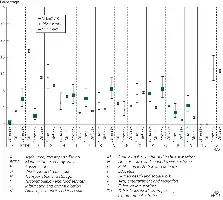
Distribution of women and men in a union, by sector of activity and under-/over-representation of women and men in same-sex unions

Note: Black borders indicate an over-representation of women (left) or men (right) in same-sex unions in the given sector, and dotted green borders indicate an under-representation. The numbers in parentheses for each sector indicate the percentage of the active population in each sector.

Source: Family and Housing survey, INSEE, 2011, weighted data.

Figure 6

Distribution of women and men in a union by occupational category and under-/over-representation of women and men in same-sex unions

Note: Black borders indicate an over-representation of women (left) or men (right) in same-sex unions in the given sector, and dotted green borders indicate an under-representation.

Source: Family and Housing survey, INSEE, 2011, weighted data.

Table 5

Distribution of men and women in same-sex and different-sex-unions by gender profile of occupational categories

Interpretation: 30.7 % of women in same-sex unions work in a mixed occupational category, versus 20.6% of women in different-sex unions.

Source: Family and Housing survey, INSEE, 2011, weighted data.

Table 6

Distribution of men and women in same-sex and different-sex-unions by gender profile of occupational categories and by level of education (%)

Coverage: Women and men aged 25-59 in a same-sex or different-sex union.

Source: Family and Housing Survey, INSEE, 2011.

Tableau

NAF code by sex and type of union, after matching

Coverage: Women and men aged 25-59 in same-sex unions, matched with individuals in different-sex unions with similar characteristics.

Source: Family and Housing survey, INSEE, 2011, weighted data.

Tableau

Occupational category by type of union, after matching

Coverage: Women and men aged 25-59 in same-sex unions, matched with individuals in different-sex unions with similar characteristics.

Source: Family and Housing survey, INSEE, 2011, weighted data.

Table A.1

Post-secondary qualification by type of union, age group (%), and hazard ratio

Interpretation: 43.8% of women aged 45-59 in a same-sex union have a post-secondary qualification (bachelor’s degree or higher). These women more often have a post-secondary qualification than women of the same age group in different-sex unions (HR = 2.44).

Source: Family and Housing survey, INSEE 2001, weighted data.

Table A.2

Factors associated with being in a same-sex (versus different-sex) union, (odds ratios)

Interpretation: A statistically significant odds ratio (higher than 1) indicates that for the modality studied, when compared to the reference modality of the variable under consideration, the factor increases the chances of belonging to the modelled group. The further the odds ratio is from 1, the greater the influence of the factor in question.

Source: Family and Housing survey, INSEE 2011, weighted data.

Tableau

Table 1. Distribution of individual characteristics at arrival and of training activities during the first four years of residence, by gender

Tableau

Table 2. Occupational field of first job and of first job corresponding to pre-migration level of education, by gender

Figure

Figure 1. Proportion (%) of immigrants without a first job, or a first job matching their pre-migration skill level, by time since arrival and gender

Source: Enquête sur les travailleurs sélectionnés, Quebec, 2002.

Figure

Figure 2. Proportion (%) of immigrants without a first job matching their pre-migration skill level, by region of origin and gender

Source: Enquête sur les travailleurs sélectionnés, Quebec, 2002.

Tableau

Table 3. Relative risks of access to a first job, by gender

Figure

Figure 3. Proportion (%) of persons without a first job, by time since arrival, gender and level of knowledge of French at arrival

Source: Enquête sur les travailleurs sélectionnés, Quebec, 2002.

Tableau

Table 4. Relative risk of finding a first job corresponding to the pre-migration level of education in Quebec, by gender

Tableau

Table A.1. Relative risks of access to a first job and a first job corresponding to pre-migration level of education

Tableau

Table 1. Life histories of the 1930 and 1945 cohorts, France

Tableau

Table 2. Life histories of the 1975 cohort. Three simulations (without ART), France

Tableau

Table 3. Results when ART is taken into account in the 1945 and 1975 cohorts, France

Figure

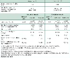
Figure 1. Proportions of the male and female population aged over 20 who completed at least primary education, Central Asia, 1900-1950

Source: Computed based on data from the1959 All-Union Census.

Figure

Figure 2. Percentage of urban population, Central Asia, 1926, 1939, 1959 censuses

Notes: * refers to Kazakskaya Autonomous Soviet Socialist Republic; ** refers to Kirghiz Soviet Socialist Republic; *** refers to Tajik Autonomous Soviet Socialist Republic.

Sources: Computed based on census data available at: http://demoscope.ru/weekly/ssp/census.php.

Figure

Figure 3. Country-level estimates of total fertility between 1910 and 2010, Central Asia

Note: The reverse survival fertility estimates based on the 1926 and 1939 censuses are five-year moving averages.

Sources: See electronic appendix for detailed data sources.

Figure

Figure 4. Ethnic-specific estimates of total fertility (children per woman), Central Asia, 1910-2010

Sources: See electronic appendices for detailed data sources and information on estimation methods.

Figure

Figure 5. Percentage of married women age 20-24 (A) and age 35-39 (B), 1939, 1959 and 1970 censuses, Central Asia

Source: Computed based on census data available at: http://demoscope.ru/weekly/ssp/census.php

Figure

Figure 6. Percentage of childless women by birth cohort, Central Asia, 1979 and 1989 censuses

Source: 1979 All-Union Census and computed based on the 1989 All-Union Census available at: http://demoscope.ru/weekly/ssp/ussr_wom_89.php

Figure

Figure 7. Percentage contribution of the change at each parity to the fertility increase among women of the titular ethnic group born in 1915-1919 and 1935-1939, Central Asia, 1979 census

Source: Computed based on data from the All-Union 1979 Census.

Figure

Figure 8. Stylized pattern of fertility change in Central Asia between 1910 and 2010

Source: Authors’ calculations.

Table 1

Means of the dependent and independent variables

Note: Standard deviations in parentheses.

Sources: (1). Authors’ calculations using Census 2011. (2). Authors’ calculations using housing micro data from Census 2011. (3). Authors’ calculations using District Level Household Survey -3 (DLHS 3). (4). Guilmoto and Rajan (2013).

Table 2

Moran’s I for the dependent and independent variables

Interpretation: Values of I range from −1 (indicating perfect dispersion) to +1 (perfect correlation). A zero value indicates a random spatial pattern.

Source: Authors’ calculations.

Figure 1