Forecasting sovereign CDS VOLATILITY: A comparison of univariate GARCH-class models
Pages 27 à 56
Citer cet article
- SABKHA, Saker,
- DE PERETTI, Christian
- et MALLEK, Sabrine,
- Sabkha, Saker.,
- et al.
- Sabkha, S.,
- De Peretti, C.
- et Mallek, S.
https://doi.org/10.3917/vse.209.0027
Citer cet article
- Sabkha, S.,
- De Peretti, C.
- et Mallek, S.
- Sabkha, Saker.,
- et al.
- SABKHA, Saker,
- DE PERETTI, Christian
- et MALLEK, Sabrine,
https://doi.org/10.3917/vse.209.0027
Notes
-
[1]
The majority of papers dealing with the predictive power of GARCH models, only focus on the major stock indexes and exchange rates (Poon, 2005).
-
[2]
For an exhaustive survey of the proposed ARCH-class models, see (Poon, 2005).
-
[3]
For a complete theoretical and empirical survey on the use of univariate ARCH processes in financial studies, see (Bollerslev, Chou et Kroner, 1992).
-
[4]
Today’s shocks on a financial asset (future contracts for example) have a significant impact on the conditional volatility several periods in the future.
-
[5]
The IGARCH(1,1) is equivalent to the Exponentially Weighted Moving Average (EWMA) model developed by (Morgan, 1996).
-
[6]
Positive and negative financial shocks revamp asymmetrically the variance. Furthermore, bad news (shocks) generate greater volatility than good news.
-
[7]
The volatility’s different reactions to signs and sizes of past innovations are also suggested in the Threshold Heteroskedastic model (TGARCH) of (Zakoian, 1994). The major difference is that in the TGARCH model the conditional standard deviation (σt) is considered rather than the conditional variance (σ2t).
-
[8]
The autocorrelation function of time series returns decreases gradually.
-
[9]
When the memory parameter, d=0, the FIEGARCH formulation is equivalent to the conventional EGARCH(1,1) (FIEGARCH(1,0,1) ≃ EGARCH(1,1)).
-
[10]
When d of the HYGARCH is positive, it is considered as a unit root process.
-
[11]
(Diebold, 2015) argue that allowing for forecast errors to be non-Gaussian, nonzero mean and autocorrelated produces better tests’ results.
-
[12]
More methods exist in the literature to proxy the volatility of financial assets, such as the high-low measure and the realized volatility estimate. For a complete survey of these methods, see (Poon, 2005).
-
[13]
Another commonly used long-range test is the Gaussian semi-parametric (GSP) (Robinson, 1995). Results of the GSP are not reported here but they are similar to those of the GPH.
-
[14]
Other statistical distributions should, as well, be considered in further studies, such as the Skewed t-student…
-
[15]
According to (Pan et Fang, 2012), the ML and the GLS give the same estimators in only one special case, that is Rao’s simple covariance structure.
-
[16]
Maximizing the likelihood function means that the number of available observations tends towards infinity, then the estimator
correspond to their true values Ω.
-
[17]
See (Fletcher, 2013), for example, for an exhaustive survey on the different aspects (unconstrained and constrained) of optimization methods used in solving mathematical functions and the way they empirically perform.
Introduction
1Understanding the fluctuations’ dynamic of financial assets has always been of a particular interest in the academic and non-academic spheres. The considerable number of studies focusing on the stock prices’ mechanism point out several stylized facts characterizing the financial markets such as: the volatility clustering, the non-stationarity… (See (Niu et Wang, 2013) for example for a study of the statistical behaviors of the Shanghai Composite Index and Hang Seng Index). Besides the stock markets widely studied, analyzing the characteristics of the credit market, and particularly the sovereign CDS market, is likewise interesting especially when it comes to investigating the impact of financial properties on the suitability of the CDS volatility modeling and forecasting ability. The curious increase in the empirical studies dealing with modeling CDS data during the last decade can be explained by several reasons: (i) the constantly evolving outstanding amount of the CDS contracts reaching its highest values during the crisis periods, (ii) the need of more clear understanding of the role played by this market in the spread of crises and (iii) and the requirement of identifying the main explaining factors of credit risk. Furthermore, the use of CDS contracts no more as hedging instruments but rather as diversification, trading and speculation instruments has legitimized the usefulness of CDS volatility forecasting to investors for both risk management and portfolio management.
2Despite the relevance of the volatility forecasts particularly in the decision process and considering the grown interest in predicting credit spreads, the nonexistence of papers in the literature of CDS spreads dealing with the ability of GARCH models to accurately forecast the volatility of the CDS is completely outrageous [1]. The literature on CDS is mainly composed by studies that focus on the determinants of these credit spreads (Costantini, Fragetta et Melina, 2014 ; Fontana et Scheicher, 2016 ; Oliveira, Curto et Nunes, 2012) or the Granger Causal relationship between CDS markets and related markets (Coudert et Gex, 2010, 2013 ; Longstaff et al., 2011 ; Sabkha, de Peretti et Mezzez, 2019). The very few papers that investigate the forecasts of CDS spreads (Avino et Nneji, 2014 ; Krishnan, Ritchken et Thomson, 2010 ; Sharma et Thuraisamy, 2013 ; Srivastava et al., 2016) only focus on the first moment order, while the predictability of the CDS volatility remains understudied. Yet, these studies try to forecast the CDS spreads based on the commonly known economic and financial determinants and not based on the predictive ability of the econometric models. Considering the foregoing gaps, this study aims to extent the literature by investigating the forecasting performance of 9 GARCH-class models in the sovereign CDS markets from January 2nd, 2006 to March 31st, 2017.
3Our study contributes to the existing literature in several ways: first, as far a we are concerned, none of the previous studies has focused on the predictability of CDS volatility, especially when it comes to the sovereign market. Second, our paper contributes as well to the literature by implementing a larger set of statistical loss function criteria -taking into account the nonzero mean and the heteroscedasticity of the forecast errors - to assess the out-of-sample predictive ability of the models in comparison with existing forecasting papers on financial assets. Third, the comparative study between linear and non-linear ARCH-class models provides a better and clearer comprehension of the in-sample and out-of-sample fit of the CDS data. Finally, our data set allows us to draw more robust and worldwide conclusions, as it is composed by CDS spreads for 38 countries from all over the world covering the two economic and financial recent crises when the volatility of asset prices have reached their highest unexpected levels. Our empirical findings show that the sovereign CDS market is characterized by the same stylized facts as the stock market: volatility clustering, leverage effects and long memory behavior. The results of the diagnostic tests on the in-sample modeling generally show that no model outperforms all the others in terms of fitting. Based on the results the 7 loss functions, the predictive performance of the fractionally-integrated models seems to be more accurate, emphasizing the importance of taking into account the long-range memory and the nonlinear behavior of CDS spreads while forecasting volatility. Among the fractionally-integrated models, our results show that the FIGARCH and the FIEGARCH are the most accurate models, providing the best out-of-sample performances in most cases. The rest of the paper is organized as follows. A brief literature review of the previous studies predicting financial assets is presented in Section 1. Section 2 presents the sample and data used to compare the predictive ability and displays the 9 volatility forecasting models under focus. Results of the in-sample and out-of-sample analysis are reported is Section 3. Section 4 concludes the paper.
1 – Literature review
4Investigating the degree to which financial time series can be accurately forecasted, has always been in the limelight of researchers’ issues. The empirical literature on the modeling and predicting volatility processes is extensive and takes into account more and more financial markets properties. (Engle, 1982) is the first researcher to model financial data through a time-varying stochastic process characterized by a nonconstant correlated variance so-called ARCH model. A generalization of this Autoregressive Conditional Heteroscedaticity model is then proposed by (Bollerslev, 1986) with more parsimonious and less overparametrization and biasedness in the estimates. Some extensions of this model are afterwards proposed, taking into account more stylized facts of the financial markets: leverage effects (Glosten, Jagannathan et Runkle, 1993 ; Nelson, 1991), stationarity issues (Engle et Bollerslev, 1986), long memory (Baillie, Bollerslev et Mikkelsen, 1996 ; Bollerslev et Ole Mikkelsen, 1996 ; Davidson, 2004 ; Ding, Granger et Engle, 1993 ; Tse, 1998) [2]… These GARCH-class volatility models have been widely used to forecast various financial data, based on their predictive power. The great focus in these studies has been primarily given to stock returns (Ferreira et Santa-Clara, 2011 ; Guidolin et al., 2009 ; Keim et Stambaugh, 1986 ; Niu et Wang, 2013 ; Poon, 2005), in which recent past information is found to help forecast the future variance. Similar studies are conducted using commodity market data, especially oil data (Agnolucci, 2009 ; Charles et Darné, 2017 ; Chkili, Hammoudeh et Nguyen, 2014 ; Wei, Wang et Huang, 2010).
5Generally, these studies show that no model outperforms all the others in capturing the time series financial and statistical features, while the non-linear GARCH-class models are found to be more relevant in terms of forecasting accuracy [3]. Unlike stock markets, exchange rates and oil market data, not many studies have been conducted to assess the predictive performance of the volatility GARCH-type models using CDS data. Despite (Krishnan, Ritchken et Thomson, 2010), (Sharma et Thuraisamy, 2013), (Avino et Nneji, 2014) and (Srivastava et al., 2016) whose aim is to predict the future changes in the CDS spreads based on some macroeconomic and market-wide variables, the literature on CDS spreads focuses generally on the key drivers and determinants of these credit spreads (Costantini, Fragetta et Melina, 2014 ; Fontana et Scheicher, 2016 ; Oliveira, Curto et Nunes, 2012) or rather on the interaction and comovement between CDS markets and the other related financial markets (Coudert et Gex, 2010, 2013 ; Longstaff et al., 2011 ; Sabkha, de Peretti et Mezzez, 2019). Among the first authors who are interested in the prediction of credit spreads, (Krishnan, Ritchken et Thomson, 2010) built credit-spread curves, based on several macroeconomic and firm-specific variables, for 241 highly and lowly credit-risky firms from 1990 to 2005. Results show that only the information contained in the riskless yield curve significantly improve the out-of-sample forecasts. Focusing more precisely on the CDS as proxy for the credit risk level, (Sharma et Thuraisamy, 2013) investigate the forecastability of the CDS spreads of 8 Asian sovereign from 2005 to 2012.
6In-sample and out-of-sample evidences reveal that the oil price uncertainty provides valuable information for predicting the future fluctuations in the sovereign CDS spreads. (Avino et Nneji, 2014) use some economic and financial factors to investigate whether the iTraxx index spreads are predictable. Based on the results of the predictive ability of some linear (Structural OLS model and AR(1)) and non-linear (Markov-switching) models, these authors show that the daily changes in the CDS index can be predictable from the yield curve, the equity returns and the changes in the VSTOXX volatility index.
7Using an error correction model before, during and after the subprime crisis, (Srivastava et al., 2016) show that the VIX predicts the future changes in 98% of the studied sovereign CDS markets. These few studies on the forecastability of CDS spreads rely on the information contained in the theoretical determinants - widely used in the empirical literature - and its ability to predict future fluctuations in the CDS market. Yet, the accuracy of these CDS predictions is assessed through some loss function criteria that are subject to nonzero mean noise and serial correlation (such as RMSE, MAE…). Furthermore, the data studied so far only cover the period of the subprime crisis and end before or right after the outbreak of the Sovereign Debt Crisis, which is quite a weak point given that all the unexpected changes in the market behavior are not taken into account in their forecasting models. Finally, the most important shortcoming of the aforementioned studies, is that they focus on the first moment order and neglect the variance in forecasting the CDS spreads.
2 – Data and methodology
8This section introduces one of our paper contributions: the sample under study, composed by countries around the world, allowing us to provide international evidences and data time line covering both the recent two financial and economic crises. Volatility forecasting models are as well presented in this section.
2.1 – Sample and data description
9Our study focuses on a sample composed by 38 worldwide countries belonging to five different geographical areas: Eastern and Western Europe, North and South America and Asia. Besides the developed countries and the emerging countries, the sample under study in this paper includes some Newly Industrialized Countries (such as Brazil, Mexico, Philippines and Thailand…) and some low economic growth countries with the highest credit risk levels (such as Portugal, Ireland, Greece and Spain…). The sample details with the economic and geographical status of each country are given in Table 1. The dataset used is composed by daily 5-year sovereign CDS spreads, denominated in US dollars and collected from Thomson Reuters. The extracted series cover a period spanning from January 2006 to March 2017, during which the world financial and credit markets have been affected by two major crises, namely the Global Financial Crisis and the Sovereign Debt Crisis. Thus, modeling that forecasts the CDS volatility and compares performances’ models are particularly interesting during this period. Indeed we observed during this period some unexpected fluctuations on the credit market.
Sample and countries ranking into economic categories and geographical positions

Sample and countries ranking into economic categories and geographical positions
The countries’ economic classification is made according to the NU, the CIA World Factbook, the IMF and the World Bank criteria, in order to have a sample with a sufficient number of countries in each category.2.2 – Marginal volatility processes: univariate ARCH-type models
10The financial markets are generally characterized by periods of volatility clustering, during which the assets’ second moment order remains high before regaining its normal levels. (Engle, 1982) proposes an Autoregressive Conditional Heteroscedasticity (ARCH) model able to capture such financial phenomenon. This volatility persistence is as well observed in the Credit Default Swap market and the use of ARCH-class models to model the variance of the CDS spreads is thus legitimate. As an extension of the ARCH model, (Bollerslev, 1986) proposes a generalized high-order ARCH process that is more parsimonious and allows for less overparametrization and biasedness in the estimates. This GARCH model is given by:

12with xt is a financial time series and μt and σt are respectively conditional mean and conditional volatility. To satisfy the positive-definite condition, some restrictions are imposed: p ≥ 0, q ≥ 0 and ω ≥ 0, αk ≥ 0 for k = 1, …, q, βh ≥ 0 for h = 1, …, p. For sake of simplicity and suitability, only models with process orders (p and q) equal to 1 are estimated. In fact, the simplest GARCH(1,1) specification is the most useful and fitted for financial time series (Bollerslev, 1986 ; Wei, Wang et Huang, 2010). The GARCH(1,1) process, as proposed by (Bollerslev, 1986), is given by the following formula:

14Furthermore to the previous model restrictions, α and β parameters must satisfy the condition of α + β < 1 to comply with the stationarity in the broad sense. A more restrictive version of the GARCH(1,1) is proposed by (Engle et Bollerslev, 1986) where the equivalent of the unit root in the mean is included in the variance so we can handle for the stationarity of the variance. The integrated GARCH(1,1) takes into account the persistence of conditional volatilities [4]. The main difference with the GARCH(1,1) is that the IGARCH requires the parameters α and β to respect the equality of α + β = 1. Thus, the IGARCH(1,1) [5] can be written as follows:

16Besides the aforementioned linear models, there exists some nonlinear GARCH-class of models taking into account the other financial market properties. The exponential GARCH, as proposed by (Nelson, 1991), is one of these models that accounts for the leverage effect and the asymmetry of the error distribution. While the nonnegativity of linear GARCH model is ensured by several parameters restrictions, the EGARCH model proposes another formulation allowing for a positive volatility without any restrictive constraints. The EGARCH(1,1) is expressed as follows:

18The asymmetric relation between assets’ fluctuation and volatility changes is depicted by the θ and γ representing respectively the sign and the magnitude of εt. (Glosten, Jagannathan et Runkle, 1993) propose a model that allows the sign and the amplitude of the innovations (εt) to affect the conditional volatility separately. The asymmetric leverage effect [6] is represented in the following formulation of the GJR-GARCH(1,1) [7] model:

20with It is a dummy variable equal to 0 when at is positive and 1 otherwise. The first model accounting for the long-range persistence of financial assets variance is developed by (Ding, Granger et Engle, 1993). This asymmetric power ARCH model allows the volatility to be long-memory [8]. The APARCH(1,1) model is:

22where δ depicts the Box-Cox power transformation of the conditional volatility (σt) and satisfies the condition of δ ≥ 0. A more flexible class of GARCH models is proposed by (Baillie, Bollerslev et Mikkelsen, 1996) who introduce a new feature of the unit root for the variance. In fact, the fractionally integrated GARCH model (FIGARCH) highlights the fact that - unlike stationary processes where the persistence of volatility shocks is finite - in unit root processes, the impact of lagged errors occurs at a slow hyperbolic rate of decay. The FIGARCH model allows, thus, to capture the long memory in financial volatility with a complete flexibility regarding the persistence degree. In fact, the FIGARCH(1,d,1) formulation depends on fractional integration parameter (d) as follows:

24with 0 < d < 1. When d=1, the FIGARCH (1,d,1) is equivalent to an IGARCH (1,1) where the persistence of conditional variance is supposed to be complete, while when d=0, it is rather equivalent to a GARCH(1,1) and no volatility persistence is taken into consideration. L is the lag operator and (1 − L)d is the financial fractional differencing operator. Other ARCH formulations are extended to the fractionally integrated GARCH, including asymmetric leverage effect presented in the EGARCH model. (Bollerslev et Ole Mikkelsen, 1996) propose a new class of model combining characteristics of the FIGARCH and the EGARCH models, so-called FIEGARCH (p,d,q). Financial assets’ volatility is, thus, better explained and depicted by a mean-reverting fractionally integrated process. The FIEGARCH(1,d,1) model is written as follows:

26where ϕ(L) and ψ(L) are lag polynomials, and - as in the EGARCH(1,1) [9] - g(εt) is a quantization function of information flows such as:

28An extension of the conventional fractionally integrated GARCH model is proposed by (Tse, 1998) so-called FIAPARCH(1,d,1). The new approach combines the long-range dependencies feature and the asymmetric impact of lagged positive and negative shocks on future volatility in one fractionally integrated model. The FIAPARCH(1,d,1) is written as follows:

30More recently, another linear GARCH model, called hyperbolic GARCH (HYGARCH) is proposed by (Davidson, 2004) who argues that the impact of lagged errors on the conditional variance discloses near-epoch dependence feature. The main contribution of this model is that the fractional integration parameter is negative (-d) instead of positive and that d increases rather when it approaches zero [10].The statistical properties included in the HYGARCH make it the most successful and used approach by financial practitioners in modeling time series volatility. The HYGARCH(1,d,1) is defined under the following formulation:

32The volatility estimation of the CDS log returns of the 38 countries is computed for 9 GARCH-class models taking into account, each time, different financial stylized facts such as long-run properties in the conditional mean and volatility clustering and long-memory behavior in the conditional variance. The BFGS-BOUNDS method (Broyden, 1970) is used to optimize the likelihood function rather than the conventional numerical optimization, in order to respect the parameters constraints, notably the stationary and the nonnegativity constraints. In addition to the widely used Box-Pierce tests and the LM ARCH effects test, several other diagnostic tests are conducted here, namely the Nyblom test, the adjusted Pearson goodness-of-fit test and the Residual-Based Diagnostic (as suggested by (Fantazzini, 2011)). The Joint Nyblom (Nyblom, 1989) is a stability test under the null hypothesis of parameters joint constancy over time against the alternative of parameters shift at an undefined breakpoint. According to (Palm et Vlaar, 1997), the adjusted Pearson goodness-of-fit test verifies whether the residuals’ empirical distribution matches or not the theoretical distribution (namely Gauss, Student or Generalized Error Distribution (G.E.D) depending on the country).
33The Residuals-Based Diagnostic test (Tse, 2002) checks for conditional Heteroscedasticity, by complementing and filling the gaps of the Box-Pierce Q statistics. All these univariate models are estimated through the most widely used approach: the Maximum Likelihood (ML) approach approximated under one of four assumed distributions about the residuals εt (Gauss, Student, Generalized Error Distribution and Skewed-Student). Among the several existing techniques to optimize the non-linear (log-) likelihood functions, we use in this paper the limited Broyden, Fletcher, Goldfarb and Shanno (BFGS-bounds) algorithm (Nocedal et Wright, 2006). The BFGS-bounds allows the estimated parameters (Ω) to only range between selected lower and upper boundaries, so we can impose the stationarity and the positivity of the models. A detailed discussion on the Maximum Likelihood estimation method and the numerical optimization algorithm used in this paper is presented in Appendix B.
2.3 – Loss function criteria
34Following (Wei, Wang et Huang, 2010), the forecasting process of the CDS volatility is implemented as follows: the 38 CDS times series timeline is divided into two subperiods: the in-sample volatility estimation is conducted from January 2nd, 2006 to March 31st, 2014 (2152 observations), and the out-of-sample model forecasts concern the last three years, i.e. from April 1st, 2014 to March 31st, 2017 (783 observations). The twenty-day out-of-sample forecasting are used to assess and compare the predictive performance of the 9 studied models. The comparison of the volatility models’ forecasting ability is not straightforward. Several measures of the predictive ability are suggested in the literature based on some loss functions. According to (Poon, 2005), (Wei, Wang et Huang, 2010) and (Pilbeam et Langeland, 2015), we cannot conclude with certainty the superiority of one model over another in terms of forecasting performance, based solely on the result of a single error statistic since each criterion may be more and less relevant from one case to another [11]. That’s why the conclusions made in this study are based on the results of a rich set of statistics composed by the 7 most popular and relevant ones, including:
- The Mean Square Error (MSE):

- The Mean Absolute Error (MAE):

- The Heteroscedatiscity-adjusted Mean Square Error (HMSE). As suggested by (Andersen, Bollerslev et Lange, 1999), the HMSE is calculated as follows:

- The Heteroscedatiscity-adjusted Mean Absolute Error (HMAE). (Bollerslev et Ghysels, 1996) proposes a loss function that better accommodates the heteroskedasticity in the forecast bias. The HMAE is calculated as follows:

- The QLIKE loss function (QLIKE). This is a test of forecast bias implied by a Gaussian likelihood (see (Wei, Wang et Huang, 2010) for further details):

- The R 2LOG loss function (R 2LOG): This loss function assesses the goodness-of-fit of the out-of-sample forecasts, based on the regressions of (Mincer, 1969):

- The Mean Logarithm of Absolute Errors (MLAE): As proposed by (Pagan et Schwert, 1990), the MLAE criterion is written as follows:

48With N is the number of predicted data and 
3 – Empirical results
49This section presents the summary statistics of the 38 studied time series. The modeling, estimation and testing of the forecasting ability of the 9 GARCH-class models are presented, as well, in this section.
3.1 – Descriptive statistics
50Descriptive statistics, displayed in Table 2, show that the studied countries present dissimilar credit risk levels with CDS spreads ranging from 1 bp to 37081.41 bp. The average daily spreads highlights, as well, this divergence in sovereign financing conditions with the largest value recorded, as expected, in Greece (9508.85 bp) and the smallest value recorded in the USA (24.01 bp). The high levels of standard deviations reveal, on the other side, that the worldwide financial and economic troubles impacted the public finances of the countries under study, doubtlessly with different magnitudes. The least volatile CDS market is Germany (24.50). According to the Augmented Dickey-Fuller test (Dickey et Fuller, 1981), all the time series present a unit root, implying that the CDS spreads of the 38 countries are non-stationary at 5% statistical level at least.
Descriptive statistics and ARCH effect tests for the CDS time series

Descriptive statistics and ARCH effect tests for the CDS time series
The table reports descriptive statistics for the daily sovereign CDS spreads of 38 countries. Min., Max. and Std. Dev. denote respectively the minimum, the maximum and the standard deviation. The Augmented-Dickey Fuller (Individual intercept included in the test equation) is a unit root test that informs about the stationary of time-series with a null hypothesis of the presence of a unit root in the process. The Engle’s ARCH-LM test with 2, 5 and 10 lag orders informs about the presence of ARCH effects in the series under the null hypothesis of no autocorrecations in the squared residuals. GPH is the log periodogram test of Geweke and Porter-Hudak (1983) with d-parameter (m=1467). This test is applied to the squared logarithmic returns (as proxy for unconditional volatility) to detect any long-range dependence volatility process. *, ** and *** refer to the statistical significance at respectively 10%, 5% and 1% levels.51Focusing on the evolution of the CDS log returns (computed as 
Daily CDS log returns of some chosen worldwide countries

Daily CDS log returns of some chosen worldwide countries
Density estimation of some chosen worldwide countries

Density estimation of some chosen worldwide countries
3.2 – Models estimation and diagnostic tests
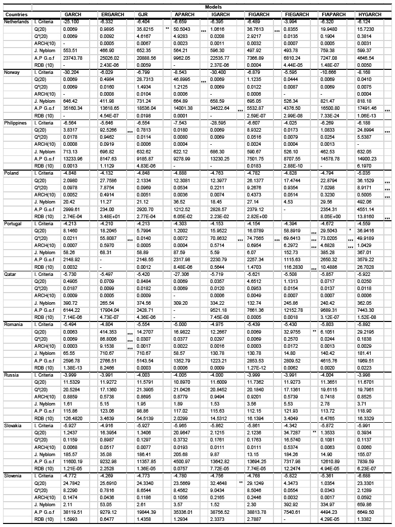
52Results of the 9 GARCH-class model estimates are not reported here but are available upon request. Even though some models are difficult to optimize, no miss-convergences are recorded for any time series. However, at first sight, the major conclusion that could be drawn regarding the models estimation process is that, taking into account several financial markets’ stylized facts (long memory characteristic, shock persistence and asymmetric leverage effects…) does not necessarily improve the models in-sample performances since the more the model is over-parametrized, the more its computation and its convergence are complicated. In fact, different inconsistency and inaccuracy of the estimator parameters in some countries and for some model can result from the complexity of the model’s statistical specifications. At the opposite, the models that great perform as to strong numerical convergence and computing-time delay are the GARCH, the IGARCH, FIGARCH and FIEGARCH. Results of the univariate misspecification tests applied on the standardized residuals are presented in Table 5 (Appendix A).
53The Q portmanteau empirical statistics with 20 lags, applied on both standardized residuals in levels and squared, show that the null hypothesis of no serial correlation is accepted in most cases, for all the studied models. The LM-ARCH test up to 10 lag orders shows, as well, that there is no heteroscdasticity in the conditional variance equations of most of time series. The GARCH, IGARCH and FIGARCH models pass this test in 100% of cases, whilst the least performant model, in terms of serial correlation, is the FIAPARCH with the presence of ARCH effects detected in 6 countries.
54Moreover, testing for conditional heteroscadticity through the Residual-Based Diagnostic (RDB) (Tse, 2002) gives better results, with absolutely no serial correlation detected in all series for the APARCH, IGARCH and FIGARCH. Based on the Nyblom test, proposed by (Nyblom, 1989), no possible shifts are detected and the parameters coefficients of the 9 models are found to be constant over time for all countries. One of the recommended steps in modeling financial data process is to evaluate the goodness of fit (D’Agostino, 1986). The fitting of our models are thus assessed, in this paper, through the adjusted Pearson goodness-of-fit test. Statistics indicate that mostly there is no difference between the empirical distributions of the residuals and the theoretical ones. Interestingly, the basic GARCH model seems to have the highest number (12 over the 38 studied series) of unconformity and discrepancy of the data from the hypothesized probability distributions. In addition to the diagnostic tests, Table 5 (Appendix A) displays the Akaike information criterion (AIC) for each model and each country.
55Results do not allow us to unanimously select only one most appropriate model. AIC results of the studied models are mitigated across the 38 countries of the sample. By minimizing the AIC, the APARCH turns out to be the best fitted model for the CDS data of 34% of the sample, while HYGARCH, IGARCH and FIAPARCH provide the best in-sample fit for respectively 26%, 18% and 11% of the studied countries. However, these results are not in line with the preliminary analysis where all the studied CDS log returns are found to be subject to long-memory feature in the variance. By only focusing in the fractionally integrated subset of models, the HYGARCH is found to majority outperform in 53% of cases, followed by the FIAPARCH in 40% of cases. These results divergence points out the limits of using the "minimizing loss of information" technique in comparing models appropriateness. Thus, this approach seems to be, in this case, not totally consistent and should only be used tentatively, at least if it is not associated with any other approaches. Hence, it is better to rather rely on the forecasting ability to select the best performant volatility model.
3.3 – Forecasting performance
56Results of the twenty-day out-of-sample volatility forecasts are reported in Table 3 and Table 4. As mentioned before, the forecasting robustness and reliability of the 9 models is studied through 7 error statistics, namely the MSE, MAE, HMSE, HMAE, QLIKE, R 2LOG and MLAE.
Results of the loss function criteria for the twenty-day out-of-sample volatility predictions

Results of the loss function criteria for the twenty-day out-of-sample volatility predictions
For all resultats, contact the authors.Summary of the number of selected models according to each criterion

Summary of the number of selected models according to each criterion
57Even though there is no unanimous dominant model in terms of forecasting ability according to all the comparison measure, it is clearly seen that the fractionally-integrated class of model outperforms the basic GARCH models - not taking into account long-memory in volatility process. Ranked in the last position by 5 out of the 7 criteria, the least forecasting performant model for CDS volatility is the EGARCH with the largest recorded errors. The lowest values of MSE, MAE and R 2LOG are recorded for the FIGARCH, whilst the lowest values of HMSE, QLIKE and MLAE are reported for the FIEGARCH, making them preferable, in terms of accurate forecasting abilities, to the other studied models. At the opposite, and according to the results of the MSE, MAE, HMAE, R 2LOG and MLAE criteria, the HYGARCH produce the highest errors, probably due to its computational complexity. These findings empirically reveal the nonlinear predictability pattern of CDS volatility. In general, our results are in line with the findings of other financial markets: the non-linear GARCH-class models, that allows for leverage effects, unsymmetrical dependencies and long-range memory in the volatility model provide a more accurate in-sample performance and a more reliable out-of-sample forecasting ability. The improvement of the forecasting power of the studied models depends, thus, on their ability to capture a maximum of financial stylized facts while estimating the CDS volatility of future days.
Conclusion
58This paper aims at assessing the performances of 9 linear and non-linear volatility models. Using daily sovereign CDS data, GARCH, IGARCH, EGARCH, GJR, APARCH, FIGARCH, FIEGARCH, FIAPARCH and HYGARCH are estimated, allowing to take into account different financial markets properties such as the leverage effect, the asymmetric reaction to good and bad news and long-range persistence.
59The performance comparison being made upon several loss function criteria and several multivariate diagnostic tests, a certain number of conclusions can be drawn. First, the in-sample estimation shows that all the models almost always pass all diagnostic tests for the most cases, and that the smallest Akaike criterion does not allow us to choose only one best fitted model. Second, none of the volatility models studied in this paper is found to be more relevant than all the others in all situations, in terms of forecasting ability. The chosen model varies from one country to another and from one loss function criterion to another. Third, in most cases and according to the majority of the errors statistics criteria, the non-linear GARCH-class models, that capture the long-memory behavior, the leverage effects and the asymmetric dependencies in the volatility process are more relevant in terms of out-of-sample forecasting ability than the others. Fourth, the FIGARCH and FIEGARCH models are found to be the most relevant and robust forecasting models. Since comparing predictive performance of volatility models is of a paramount in assessing diversifiable risk, in dynamic asset pricing theory and in optimization of portfolio allocation, the economic implication of our findings concerns particularly policymakers, financial practitioners and financial market participants generally.
60The in-sample performances show that no model clearly outperforms all the others, and since the results are mitigated and differ from one country to another, no volatility model should be selected in an arbitrary way. The model selection should rather be based on the particular features of the data used and the country studied. When it comes to the forecasting performances, some models are preferable and seem to predict accurately and robustly the future volatility of the CDS market. Thus, after taking into account the transaction costs, investors can eventually take advantage of the market’s relative inefficiency and generate extra-profits by putting in place a simple trading strategy exploiting the predictability of sovereign CDS volatility. Finally, our study shows that improving the volatility forecasts needs including the maximum of CDS market’s stylized facts.
61However, in practice, the implementation of complex models generates additional costs that are not necessarily reflected in our comparison method, which may controvert the usefulness of using better volatility predictive models. Our research line can be pursued in several ways. First, a further investigation on the performance of the volatility models can be done by carrying out a comparative study based on the superior predictive ability test rather than on the diagnostic tests and loss function criteria as in our case. We can also use information ratios based on a trading strategy (Sharpe ratio) as an alternative to these statistic criteria. Second, it would be interesting to reevaluate the forecasting performance of these different models when the estimation of the models’ parameters is carried out on a sliding window. Third, our study can be applied to the corporate CDS market, in order to assess whether the nature of the reference entity impacts the performances of the studied models. Fourth, since there is a dynamic segmentation in financial markets, it can be interesting to check the robustness of our findings using a different sample from other regions and/or a CD-term structure with different maturities.
Post-estimation diagnostic tests
Results of the diagnostic tests for the 38 worlwide countries

Results of the diagnostic tests for the 38 worlwide countries


Maximum likelihood estimation
62(Pan et Fang, 2012) argue that the Generalized Least Square (GLS)-based inference holds statistical consistency and asymptotically normal distribution for the ordinary univariate models. However, this guideline becomes inaccurate and complicated when it comes to more sophisticated regression models. Therefore, since most of our studied models are non-linear, we base the estimation of the regression coefficients on the Maximum Likelihood (ML) rather than on the linear Generalized Least Square estimate [15]. The likelihood-based determination of our models’ coefficients (Ω) is considered as follows:

64Where L(Ω) is the Likelihood Function and 
65The quasi-maximum likelihood estimator could have been consistent in estimating our conditional mean and conditional variance equations if the residuals of our time series had been normally distributed (Bollerslev et Wooldridge, 1992). However, CDS series’ innovations do not necessarily follow a Gaussian distribution and the maximum likelihood is thus better adapted. In fact, financial time series are characterized by a departure from normality with a high observed kurtosis (as stated by (Palm et Vlaar, 1997)), and the use of fat-tailed distributions is therefore more consistent.
66The log-likelihood function can be expressed in four ways following the innovations’ distribution assumptions (Gauss, Student, GED, Skewed Student).

68With T is the number of observations.

70With v is the number of the degrees of freedom.

72Where 

74With ξ denotes the asymmetry parameter, 

75As already mentioned, all the above-written functions take into account (except the log-likelihood function with ε following a Gaussian distribution, LGauss) take into account the large kurtosis properties of the CDS series, however, only the LSkewed - Student function considers for the asymmetry of the probability distribution.
76Several numerical optimization algorithms exist in the literature to solve nonlinear functions: BHHH (Berndt, Hall et Hall, 1974), BFGS (Broyden, 1970), MaxSA (Goffe, Ferrier et Rogers, 1994), BFGS-Bounds (Nocedal et Wright, 2006).
77The Berndt-Hall-Hall-Hausman (BHHH) algorithm is an iterative nonlinear equivalent to the Gauss-Newton algorithm, that is only adequate to maximize least-square functions with no strong interactions between parameters. The BHHH is consequently highly inefficient in our case. Contrary to the previous algorithm, the Broyden, Fletcher, Goldfarb and Shanno (BFGS) - based on the quasi-Newton methods - is able to solve real-valued functions. According to (Lawrence et Tits, 2001), this numerical technique solves the (log-)likelihood functions in an iterative way by allowing the parameters values (Ω) to range in the interval] − ∞, +∞[. A more restrictive version of the BFGS is used to estimate the GARCH-class models in this paper, so-called BFGS-bounds, in which the Ω estimated values are restrained to a smaller interval. (Lawrence et Tits, 2001) propose an algorithm is which the maximization is established through a sequential quadratic programming technique and conducted under some non-linear constraints, so we can control the stationarity of the models and the positivity of some parameters during the estimation. The same problem is treated in (Yuan et Lu, 2011). The authors improve the effectiveness of the optimization techniques by imposing a lower and an upper boundaries between which the parameters can possibly range at each iteraqation, enforcing all iterations and the model convergence to be feasible, as well, for a large-scale dataset. Finally, optimizing non-smooth functions with possible multiple local maxima can be conducted through a Simulated Annealing algorithm, so-called MaxSA. The robustness of this algorithm is justified by the fact that it allows to easily distinguish between local and global optima while maximizing difficult functions (Goffe, 1995) [17]. Even though the latter numerical optimization program seems to be relevant in our case, it has not been used since it doesn’t properly converge in most cases.
78In fact, in practice, the estimated model may not converge conveniently due to some optimization problems. The FIAPARCH is the most complicated models with the highest number of direct miss-convergences: either the L(Ω, Λ) function cannot reach a supremum belonging to Ω and no maximum estimate is found or at the opposite, the optimization algorithm finds several values that maximize the function.
References
- Agnolucci P. (2009), Volatility in crude oil futures: A comparison of the predictive ability of GARCH and implied volatility models, Energy Economics, vol 31, n° 2, pp. 316-321.
- Aldrich J. (1997), R.A. Fisher and the making of maximum likelihood 1912-1922, Statistical Science, vol 12, n° 3, pp. 162-176.
- Andersen T.G., Bollerslev T., Lange S. (1999), Forecasting financial market volatility: Sample frequency vis-à-vis forecast horizon, Journal of Empirical Finance, vol 6, n° 5, pp. 457-477.
- Avino D., Nneji O. (2014), Are CDS spreads predictable? An analysis of linear and non-linear forecasting models, International Review of Financial Analysis, vol 34, pp. 262-274.
- Baillie R.T., Bollerslev T., Mikkelsen H.O. (1996), Fractionally integrated generalized autoregressive conditional heteroskedasticity, Journal of Econometrics, vol 74, n° 1, pp. 3-30.
- Berndt E. R., Hall B. H., Hall R. E., Hausman J. A. (1974), Estimation and inference in nonlinear structural models. Annals of Economic and Social Measurement, vol 3, n° 4, pp. 653-665.
- Bollerslev T. (1986), Generalized autoregressive conditional heteroskedasticity, Journal of Econometrics, vol 31, n° 3, pp. 307-327.
- Bollerslev T., Chou R.Y., Kroner K.F. (1992), ARCH modeling in finance: A review of the theory and empirical evidence, Journal of Econometrics, vol 52, n° 1, pp. 5-59.
- Bollerslev T., Ghysels E. (1996), Periodic Autoregressive Conditional Heteroscedasticity, Journal of Business & Economic Statistics, vol 14, n° 2, pp. 139-151.
- Bollerslev T., Ole Mikkelsen H. (1996), Modeling and pricing long memory in stock market volatility, Journal of Econometrics, vol 73, n° 1, pp. 151-184.
- Bollerslev T., Wooldridge J.M. (1992), Quasi-maximum likelihood estimation and inference in dynamic models with time-varying covariances, Econometric Reviews, vol 11, n° 2, pp. 143-172.
- Broyden C.G. (1970), The Convergence of a Class of Double-rank Minimization Algorithms 1. General Considerations, IMA Journal of Applied Mathematics, vol 6, n° 1, pp. 76-90.
- Charles A., Darné O. (2017), Forecasting crude-oil market volatility: Further evidence with jumps, Energy Economics, vol 67, pp. 508-519.
- Chkili W., Hammoudeh S., Nguyen D.K. (2014), Volatility forecasting and risk management for commodity markets in the presence of asymmetry and long memory, Energy Economics, vol 41, pp. 1-18.
- Costantini M., Fragetta M., Melina G. (2014), Determinants of sovereign bond yield spreads in the EMU: An optimal currency area perspective, European Economic Review, vol 70, pp. 337-349.
- Coudert V., Gex M. (2010), Credit default swap and bond markets: which leads the other?, Financial Stability Review, n° 14, pp. 161-167.
- Coudert V., Gex M. (2013), The Interactions between the Credit Default Swap and the Bond Markets in Financial Turmoil, Review of International Economics, vol 21, n° 3, pp. 492-505.
- D’Agostino R.B. (1986), Goodness-of-Fit-Techniques, CRC Press.
- Davidson J. (2004), Moment and Memory Properties of Linear Conditional Heteroscedasticity Models, and a New Model », Journal of Business & Economic Statistics, 22, n° 1, pp. 16-29.
- Dickey D.A., Fuller W.A. (1981), Likelihood Ratio Statistics for Autoregressive Time Series with a Unit Root, Econometrica, vol 49, n° 4, pp. 1057-1072.
- Diebold F.X. (2015), Comparing Predictive Accuracy, Twenty Years Later: A Personal Perspective on the Use and Abuse of Diebold-Mariano Tests, Journal of Business & Economic Statistics, vol 33, n° 1, pp. 1-1.
- Ding Z., Granger C.W.J., Engle R.F. (1993), A long memory property of stock market returns and a new model, Journal of Empirical Finance, vol 1, n° 1, pp. 83-106.
- Engle R.F. (1982), Autoregressive Conditional Heteroscedasticity with Estimates of the Variance of United Kingdom Inflation, Econometrica, vol 50, n° 4, pp. 987-1007.
- Engle R.F., Bollerslev T. (1986), Modelling the persistence of conditional variances, Econometric Reviews, vol 5, n° 1, pp. 1-50.
- Fantazzini D. (2011), Fractionally Integrated Models for Volatility: A Review, in Gregoriou G.N., Pascalau R. (dirs.), Nonlinear Financial Econometrics: Markov Switching Models, Persistence and Nonlinear Cointegration, Palgrave Macmillan UK, London, pp. 104-123.
- Ferreira M.A., Santa-Clara P. (2011), Forecasting stock market returns: The sum of the parts is more than the whole, Journal of Financial Economics, vol 100, n° 3, pp. 514-537.
- Fletcher R. (2013), Practical Methods of Optimization, John Wiley & Sons.
- Fontana A., Scheicher M. (2016), An analysis of euro area sovereign CDS and their relation with government bonds, Journal of Banking & Finance, vol 62, pp. 126-140.
- Geweke J., Porter-Hudak S. (1983), The Estimation and Application of Long Memory Time Series Models, Journal of Time Series Analysis, vol 4, n° 4, pp. 221-238.
- Glosten L.R., Jagannathan R., Runkle D.E. (1993), On the Relation between the Expected Value and the Volatility of the Nominal Excess Return on Stocks, The Journal of Finance, vol 48, n° 5, pp. 1779-1801.
- Goffe W. (1995), Simulated Annealing-Global optimization method that distinguishes between different local optima, Website.
- Goffe W.L., Ferrier G.D., Rogers J. (1994), Global optimization of statistical functions with simulated annealing, Journal of Econometrics, vol 60, n° 1, pp. 65-99.
- Guidolin M., Hyde S., McMillan D., Ono S. (2009), Non-linear predictability in stock and bond returns: When and where is it exploitable ?, International Journal of Forecasting, vol 25, n° 2, pp. 373-399.
- Keim D.B., Stambaugh R.F. (1986), Predicting returns in the stock and bond markets, Journal of Financial Economics, vol 17, n° 2, pp. 357-390.
- Krishnan C.N.V., Ritchken P.H., Thomson J.B. (2010), Predicting credit spreads, Journal of Financial Intermediation, vol 19, n° 4, pp. 529-563.
- Lawrence C.T., Tits A.L. (2001), A Computationally Efficient Feasible Sequential Quadratic Programming Algorithm, SIAM Journal on Optimization, vol 11, n° 4, pp. 1092-1118.
- Longstaff F.A., Pan J., Pedersen L.H., Singleton K.J. (2011), How Sovereign Is Sovereign Credit Risk ?, American Economic Journal: Macroeconomics, vol 3, n° 2, pp. 75-103.
- Lopez J.A. (2001), Evaluating the predictive accuracy of volatility models, Journal of Forecasting, vol 20, n° 2, pp. 87-109.
- Mincer J.A. (1969), Economic Forecasts and Expectations: Analysis of Forecasting Behavior and Performance, National Bureau of Economic Research, Inc.
- Morgan J.P. (1996), Risk Metrics technology document, Morgan Guaranty Trust Company of New York, New York, pp. 35–65.
- Nelson D.B. (1991), Conditional Heteroskedasticity in Asset Returns: A New Approach, Econometrica, vol 59, n° 2, pp. 347-370.
- Niu H., Wang J. (2013), Volatility clustering and long memory of financial time series and financial price model, Digital Signal Processing, vol 23, n° 2, pp. 489-498.
- Nocedal J., Wright S. (2006), Numerical Optimization, Springer Science & Business Media. New York.
- Nyblom J. (1989), Testing for the Constancy of Parameters over Time, Journal of the American Statistical Association, vol 84, n° 405, pp. 223-230.
- Oliveira L., Curto J.D., Nunes J.P. (2012), The determinants of sovereign credit spread changes in the Euro-zone, Journal of International Financial Markets, Institutions and Money, vol 22, n° 2, pp. 278-304.
- Pagan A.R., Schwert G.W. (1990), Alternative models for conditional stock volatility, Journal of Econometrics, vol 45, n° 1, pp. 267-290.
- Palm F.C., Vlaar P.J. (1997), Simple diagnostic procedures for modeling financial time series, Maastricht University.
- Pan J.-X., Fang K.-T. (2012), Growth Curve Models and Statistical Diagnostics, Springer Science & Business Media.
- Pilbeam K., Langeland K.N. (2015), Forecasting exchange rate volatility: GARCH models versus implied volatility forecasts, International Economics and Economic Policy, vol 12, n° 1, pp. 127-142.
- Poon S.-H. (2005), A Practical Guide to Forecasting Financial Market Volatility, John Wiley & Sons.
- Robinson P.M. (1995), Log-Periodogram Regression of Time Series with Long Range Dependence, The Annals of Statistics, vol 23, n° 3, pp. 1048-1072.
- Sabkha S., de Peretti C. de, Mezzez H. (2019), International risk spillover in sovereign credit markets: an empirical analysis, Managerial Finance, vol 45, n° 8, pp. 1020-1040.
- Sharma S.S., Thuraisamy K. (2013), Oil price uncertainty and sovereign risk: Evidence from Asian economies, Journal of Asian Economics, vol 28, pp. 51-57.
- Srivastava S., Lin H., Premachandra I.M., Roberts H. (2016), Global risk spillover and the predictability of sovereign CDS spread: International evidence, International Review of Economics & Finance, vol 41, pp. 371-390.
- Tse Y.K. (1998), The conditional heteroscedasticity of the yen–dollar exchange rate, Journal of Applied Econometrics, vol 13, n° 1, pp. 49-55.
- Tse Y.K. (2002), Residual-based diagnostics for conditional heteroscedasticity models, The Econometrics Journal, vol 5, n° 2, pp. 358-373.
- Wei Y., Wang Y., Huang D. (2010), Forecasting crude oil market volatility: Further evidence using GARCH-class models, Energy Economics, vol 32, n° 6, pp. 1477-1484.
- Yuan G., Lu X. (2011), An active set limited memory BFGS algorithm for bound constrained optimization, Applied Mathematical Modelling, vol 35, n° 7, pp. 3561-3573.
- Zakoian J.-M. (1994), Threshold heteroskedastic models, Journal of Economic Dynamics and Control, vol 18, n° 5, pp. 931-955.
Mots-clés éditeurs : critères des fonctions de perte, modèles de prévision, prévisibilité, volatilité du CDS
Date de mise en ligne : 23/06/2020
https://doi.org/10.3917/vse.209.0027